6. TSG

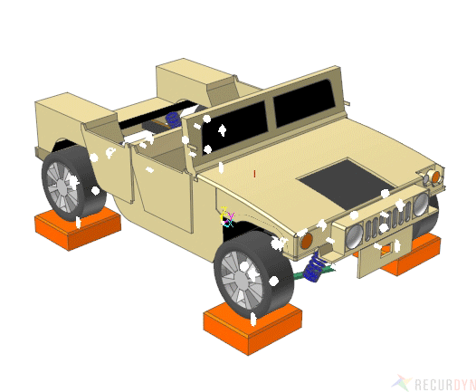
TSG example

RecurDyn/TSG (Time Signal Generator) is a toolkit that generates the Input Signals which can be applied to MBD or MFBD model. In other words, if the Target Signals are obtained, which are measured as accelerations, velocities, displacements, and so on at the specific locations of a physical model through the experimental test, RecurDyn/TSG can find out the Input Signals to match the Target Signals.

6.1. TSG Overview

RecurDyn/TSG (Time Signal Generator) generates Input Signals by using the signal processing. After the Target Signals are obtained such as accelerations, velocities, displacements, and so on at the specific locations of a physical model in the experimental test, RecurDyn/TSG can find out Input Signals so that the Target Signals can be matched after simulation. After that, the Input Signals can be applied to Forces or Motions (displacement, velocity, acceleration) as function expressions in the MBD model.

In experimental test, test engineers can measure Experiment Data such as accelerations, forces, angular position and displacements at some location of the structure. However, the measured data can’t be applied directly to the MBD model in RecurDyn because the MBD model can’t be built considering all non-linear properties of physical model. That means that the MBD model is different with the physical model. Therefore, it is needed to calculate the new Input Signals of the MBD model in order to match the measured signals of the physical model. If the Output Signals of MBD are similar to the measured signals after applying the new Input Signal to the MBD model, the MBD Model can guarantee the similar model compared to the physical model.

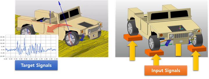
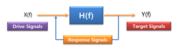
Target Signals and Input Signals

TSG Terminology

• Target Signals are user-defined signals that we want to reproduce and that has been measured experimentally.

• Response Signals are Output Signals of RecurDyn at the location of the virtual Sensors during iterative simulation. These signals at the end of the process have to match the Target Signals.

• Drive Signals are Input Signals of MBD model at the location of the virtual Actuators.

• Actuator Defines Drive Signal Locations applied to Motion or Force on the Joint or Force elements on a MBD Model.

• Sensor Defines Response Signal Locations to match user-defined Target Signals as a general Expression.

TSG Terminology

TSG Procedure

1. Set up virtual Actuators & Sensors. This implies that the user needs to define the location, type and direction of the measurement in RecurDyn.

2. Define an association between the sensors and Target Signals.

3. Calculate FRF (Frequency Response Function) after simulation.

4. Correct the drive signal iteratively using the error between Target Signals and Response Signals.

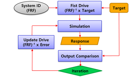
TSG Procedure flowchart

6.2. Functions for TSG

Several functions are supported to simulate TSG.

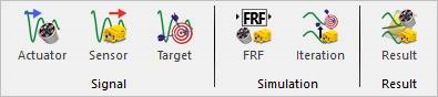
Signal, Simulation, and Result group in the TSG tab

6.2.1. Signal

You should set following three entities.

Signal group in the TSG tab

6.2.1.1. Actuator

Actuator should be created at least one to simulate. Actuator is an input of the TSG model. The concept of both TSG/Actuator and Control/Plane Input is the same.

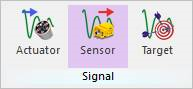
Actuator icon of the Signal group in the TSG tab

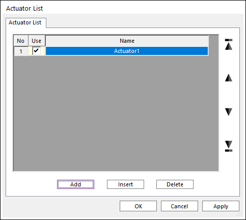
Actuator List dialog box

• Use: Determines whether or not to use.

• Name: Defines a name.

• Add: Adds a row to the end of the table.

• Insert: Inserts a row where the cursor is and move the current and later rows down.

• Delete: Deletes the row where the cursor is and move the later rows up.

Step to create an Actuator

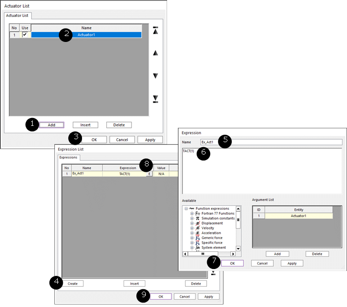
Usage of an Actuator

1. Click Add in the Actuator List dialog box.

2. Rename an actuator.

3. Select a force or a joint entity to set the actuator.

4. Click EL.

5. Click Create in Expression List dialog box.

6. Rename an Expression name.

7. Edit the actuator using “TACT(Acutator_ID)” expressions in each actuator element.

6.2.1.2. Sensor

Sensor should be created at least one to simulate. Sensor is an output of the TSG model. The concept of both TSG/Sensor and Control/Plane Output is the same.

Sensor icon of the Signal group in the TSG tab

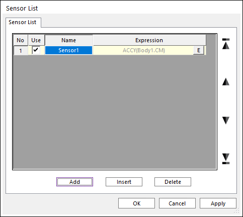
Sensor List dialog box

• Use: Determines whether or not to use.

• Name: Defines a name.

• Expression: Defines an expression function.

• Add: Adds a row to the end of the table.

• Insert: Inserts a row where the cursor is and move the current and later rows down.

• Delete: Deletes the row where the cursor is and move the later rows up.

Step to create a Sensor

Usage of a sensor

1. Click Add in Sensor List dialog box.

2. Rename an Expression name.

3. Edit an Expression.

6.2.1.3. Target

Target should be set to simulate.

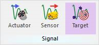
Target icon of the Signal group in the TSG tab

There are two tabs in Target Output List dialog.

• Target Output List tab: Set Target Signal by choosing a “*.TARGET” file.

• Target Output Function tab: Making “*.TARGET” file from a signal file “*.CSV”.

Step to set Target

Example to set a target

1. Move to Target Output Function tab in Target Output List dialog.

2. Select a “*.CSV” file which has the target sensor signal(s).

3. Set target output “*.TARGET” file name and path.

4. Click Create Target Output File.

5. Move to Target Output List tab in Target Output List dialog box.

6. Check loading the “*.TARGET” file or select another “*.TARGET” file.

6.2.1.3.1. Target Output List tab

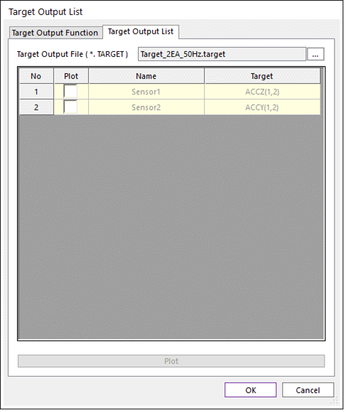
The list cannot be modified. The list is always the same with created Sensor list. Because, the Target channels should be the same with the created Sensor channels.

<Check>Figure 1 Target Output List dialog box [Target Output List tab]

• Target Output File (*.TARGET) : *.TARGET file can be set by clicking ….

• Plot: If a *.TARGET file is set and some plot check box in the list are checked, then the user can see the Target signal of choosing Sensor channel by clicking Plot.

  

  Plot example of Target Output List tab

6.2.1.3.2. Target Output Function tab

The list cannot be modified. The list is always the same with created Sensor list. Because, the Target channels should be the same with the created Sensor channels.

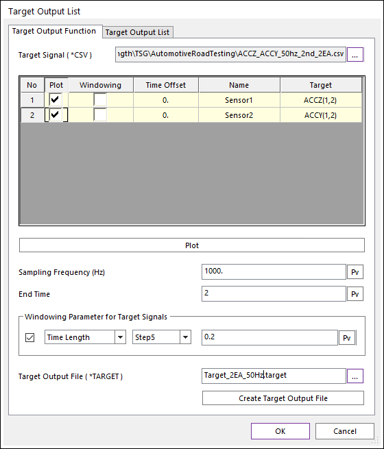
Target Output List dialog box [Target Output Function tab]

• Target Signal (*.CSV): “*.CSV” file should be needed. All data of “*.CSV” should be CSV (Comma-Separated Values). And there’s no needed header strings on first line. The number of columns should be 2 times of the number of sensors. Because every odd column should be a time data.

  

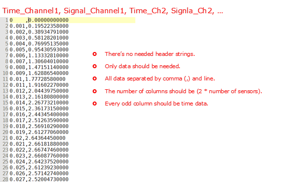
  CSV file format for Target Signal

• Plot: User can choose plot view or not.

• Windowing: If this checkbox is checked, then the generated target signal will be considered the windowing function. Default is unchecked.

• Time offset: If this value is set, then the time data of the CSV Signal will be considered as (Time_CSV-Time_Offset). Default value is 0.

• Plot: If a “*.CSV” is set and some plot check box are checked, then user can see the signal data on the opened scope dialog.

• Sampling Frequency (Hz): Sampling Frequency (Hz) should be set.

• End Time (s): End Time (s) should be set. The number of target signal data should be (Sampling_Frequency * End_Time + 1).

• Windowing Parameter for Target Signals: If the check box is selected, then a windowing function will be considered. Linear trapezoidal function is always computed.

• Data Size: A natural value greater than 0 should be set. And the Data Size should be lower than the number of signal data.

• Linear/Step5: Two interpolation function types are available for windowing function. Default is Step5 function.

• Time Length (s): A real number greater than 0.0 should be set.

  

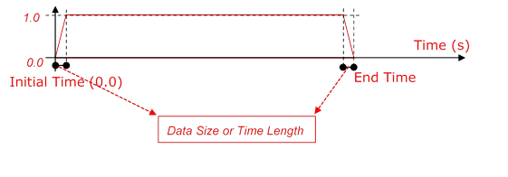
  Windowing function for generating “*.TARGET” file

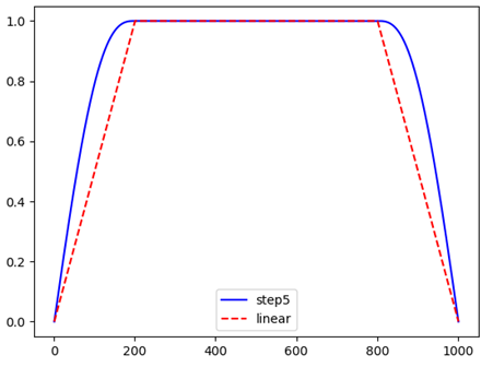
Comparison of the interpolation types for Windowing function

• Target Output File (*.TARGET): Defines a file name and path by clicking ….

• Create Target Output File: Generates the *.TARGET file by clicking this button.

6.2.2. Simulation

Simulation group in the TSG tab

6.2.2.1. FRF

FRF (Frequency Response Function) is should be needed to simulation in TSG toolkit.

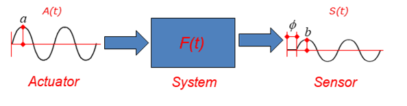
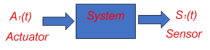
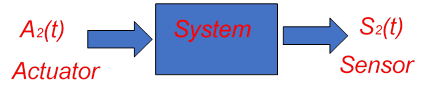
A schematic diagram of the TSG model

FRF can be computed like as <Check>equation (1) on the frequency domain.

(1)\[\begin{split}\begin{aligned} & \mathbf{F}(s)\mathbf{A}(s)=\mathbf{S}(s) \\ & \mathbf{F}(s)=\mathbf{S}(s){{\mathbf{A}}^{-1}}(s) \\ \end{aligned}\end{split}\]

Where, \(\mathbf{A}(s)\) and \(\mathbf{S}(s)\) are Actuator Signal and Sensor Signal on the frequency domain. The \(s\) means a frequency coordinate. The \(\mathbf{F}(s)\) is defined as FRF (Frequency Response Function) in the TSG.

The signals both \(\mathbf{A}(s)\) and \(\mathbf{S}(s)\) are computed using FFT (Fast Furieror Transfom).

(2)\[\begin{split}\begin{aligned} & \mathbf{A}(t)\xrightarrow{FFT}\mathbf{A}(s) \\ & \mathbf{S}(t)\xrightarrow{FFT}\mathbf{S}(s) \\ \end{aligned}\end{split}\]

After computing FRF, inverse FRF (\({{\mathbf{F}}^{-1}}(s)\)) will be computed. Generally, the inverse FRF can be computed by the Pseudo-inverse method.

FRF icon of the Simulation group in the TSG tab

There are two tabs in FRF dialog box.

• FRF tab: There are analysis options to generate FRF.

• FRF Result tab: User can check the FRF, the inverse FRF, the actuator signals and the sensor signals.

FRF dialog box

Step for computing FRF

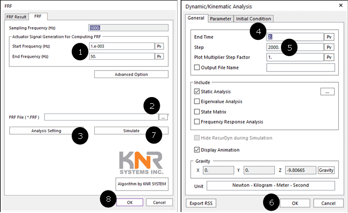
Usage FRF simulation

1. Click FRF icon.

2. Set Start and End Frequencies.

3. Click Analysis Setting.

4. Set the End Time on the Dynamic/Kinematic Analysis dialog. The End Time should be the same of the generated “*.TARGET” file.

5. Set Step on the Dynamic/Kinematic Analysis dialog. The Step should be the same with (Sampling_Frequency * End_Time).

6. Click OK to leave the Dynamic/Kinematic Analysis dialog.

7. Set FRF file name and path on the FRF dialog.

8. Click Simulation for computing FRF and generating “*.FRF” file.

6.2.2.1.1. FRF tab

All signal entities (Actuator, Sensor and, Target) should be already set to simulate FRF.

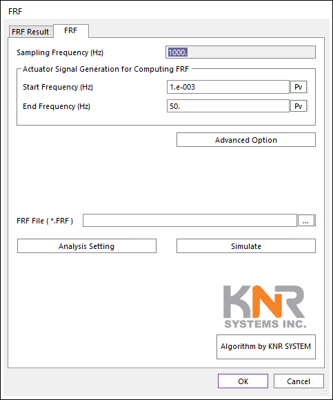
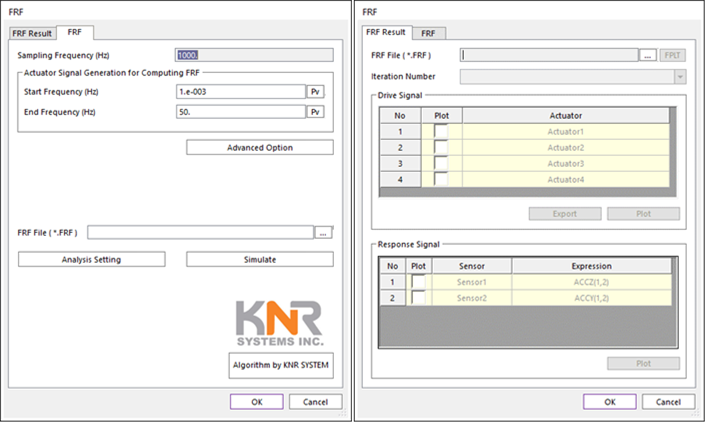
FRF dialog box [FRF tab]

• Sampling Frequency (Hz): User cannot change this value. This value is the Sampling Frequency (Hz) of loaded “*.TARGET” data.

• Actuator Signal Generation for Computing FRF: The Actuator signals (called drive signals) for computing FRF is using a Chirp signal (A sweep function) using following two parameters.

• Start Frequency (Hz): Default value is 0.01 Hz.

• End Frequency (Hz): Default value is 100.0 Hz.

  

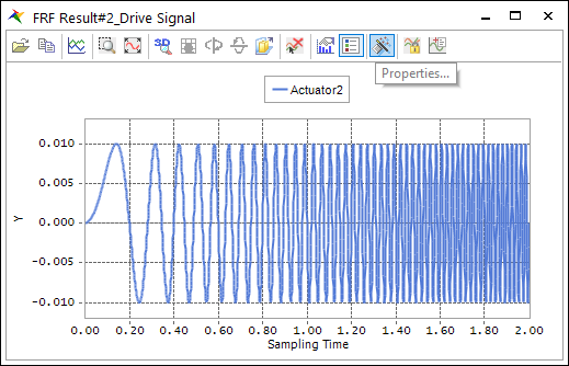
  Chirp signals

• Advanced Option: Currently user can change to magnitude data of each Actuator channels. Default magnitude is set to 1.0.

  

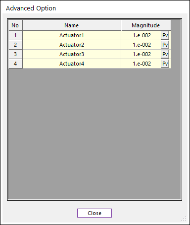
  Advanced Option dialog box

• FRF File (*.FRF): Defines a file name and path by clicking ….

• Analysis Setting: Dynamic/Kinematic Analysis dialog is opened. Because, currently TSG is only supported dynamic/kinematic analysis. The End Time and Step should be match on TSG setting.

• End Time data on the Dynamic/Kinematic Anlaysis dialog should be the same with the End Time of “*.TARGET” data.

• Step data on the Dynamic/Kinematic Anlaysis dialog should be set with (End_Time * Sampling_Frequency).

  

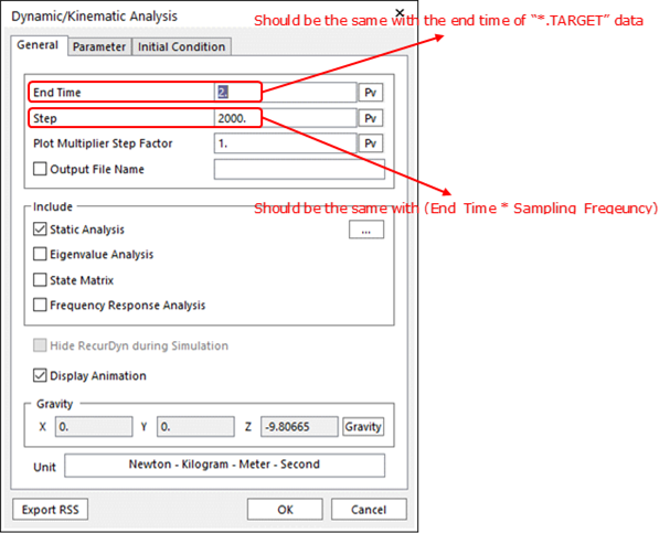
  Dynamic/Kinematic Analysis dialog

• Simulate: Computes FRF and generate “*.FRF” file.

6.2.2.1.2. FRF Result tab

Using this dialog, user can check the FRF, inverse FRF, Actuator signals and, Sensor Signals. In order to check, the “*.FRF” file is needed.

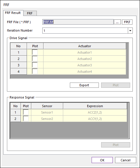
FRF dialog box [FRF Result tab]

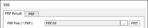
FRF File setting

• FRF File (*.FRF): Defines “*.FRF” file by clicking ….

• FPLT: Checks the FRF and the inverse FRF functions with Plot windows.

  

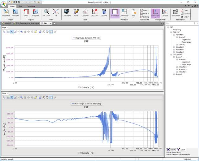
  Plot view for FRF and Inverse FRF by clicking FPLT

  

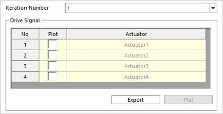
  Drive Signal region on the FRF Result tab

• Iteration Number: Defines the Iteration Number. Iteration Number means the simulation count value for computing FRF. And the Iteration Number is always the same with the number of Actuator channels.

• Drive Signal

• Plot check box in list view

• Export: Generate “*.TAI” file including the Actuator signals on time domain.

• Plot: User can see the signal data on the opened scope dialog.

  

  Response Signal region on the FRF Result tab

• Response Signal

• Plot check box in list view

• Plot: User can see the signal data on the opened scope dialog.

6.2.2.2. Iteration

Before the Iteration simulation of the TSG, the FRF simulation should be needed. Because, the Iteration simulation uses inverse FRF function.

The first drive signal \({{\mathbf{A}}_{1}}(t)\) is computed following <Check>equation (1).

(3)\[\begin{split}\begin{aligned} & \mathbf{T}(t)\xrightarrow{FFT}\mathbf{T}(s) \\ & \mathbf{T}(s){{\mathbf{F}}^{-1}}(s)={{\mathbf{A}}_{1}}(s) \\ & {{\mathbf{A}}_{1}}(s)\xrightarrow[FF{{T}^{-1}}]{}{{\mathbf{A}}_{1}}(t) \\ \end{aligned}\end{split}\]

Where, \(\mathbf{T}(t)\) and \({{\mathbf{F}}^{-1}}(s)\) are the target signals on the time domain and inverse FRF function, respectively.

First simulation of the Iteration simulation

The first simulation with the first drive signals. Then error signals (\({{\mathbf{E}}_{1}}(t)\)) of the first simulation can be computed with following <Check>equation (2).

(4)\[{{\mathbf{E}}_{1}}(t)\equiv \mathbf{T}(t)-{{\mathbf{S}}_{1}}(t)\]

The drive signal \({{\mathbf{A}}_{2}}(t)\) of the second simulation is computed following <Check>equation (3).

(5)\[\begin{split}\begin{aligned} & {{\mathbf{E}}_{1}}(t)\xrightarrow{FFT}{{\mathbf{E}}_{1}}(s) \\ & {{\mathbf{A}}_{2}}(s)={{\mathbf{A}}_{1}}(s)+{{f}_{learning}}{{\mathbf{E}}_{1}}(s){{\mathbf{F}}^{-1}}(s) \\ & {{\mathbf{A}}_{2}}(s)\xrightarrow[FF{{T}^{-1}}]{}{{\mathbf{A}}_{2}}(t) \\ \end{aligned}\end{split}\]

Where, \({{f}_{learning}}\) is a scalar value and called a learning factor. The learning factor cannot be 0.0.

Second simulation of the Iteration simulation

After second simulation, we can compute the second error signals \({{\mathbf{E}}_{2}}(t)\) again.

(6)\[{{\mathbf{E}}_{2}}(t)\equiv \mathbf{T}(t)-{{\mathbf{S}}_{2}}(t)\]

In the case of the other simulation step, the second simulation procedure is repeated.

Iteration icon of the Simulation group in the TSG tab

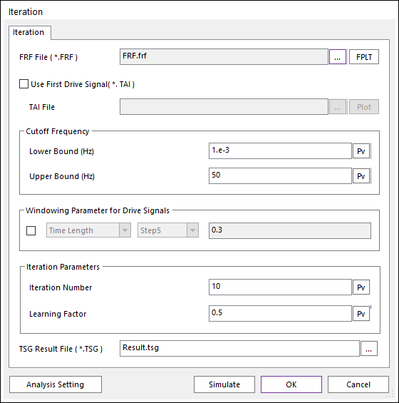
Iteration dialog box

• FRF File (*.FRF): Defines “*.FRF” file by clicking ….

• FPLT: Checks the FRF and the inverse FRF functions in the plot window.

• Use First Drive Signal (*.TAI): Default is unchecked. If this is checked, then the first drive signal is replaced the user selected signals in the input “*.TAI” file instead of <Check>equation (1).

• TAI File: If the Use First Drive Signal (*.TAI) is checked, then a “*.TAI” file should be set using “…” file. The “*.TAI” file can be generated Export function in FRF Result and Result dialogs.

• Plot: If a “*.TAI” file is selected, then User can see the signal data on the opened scope dialog.

• Cutoff Frequency: In order to ignore data of the inverse FRF this option is needed. Data of inverse FRF is between the Lower Bound and the Upper Bound frequencies is used to compute the next Drive Signal.

• Lower Bound (Hz): Default is 0.0 Hz.

• Upper Bound (Hz): Default is 1000000.0 Hz

• Windowing Parameter for Drive Signals: If the check box is selected, then a windowing function will be considered. Linear trapezoidal function is always computed.

• Data Size: A natural value greater than 0 should be set. And the Data Size should be lower than the number of signal data.

• Linear/Step5 : Two interpolation function types are available for windowing function.

• Time Length (s): A real number greater than 0.0 should be set.

  

  Windowing function for the Iteration simulation

Comparison of the interpolation types for Windowing function

• Iteration Parameters

• Iteration Number: The simulation is repeated with the Iteration Number. Default is 1.

• Learning Factor: User can modify the learning factor \({{f}_{learning}}\) of <Check>equation (3). Default is 0.5. The range of the Learning Factor: \(0.0<{{f}_{learning}}\le 1.0\).

• TSG Result File (*.TSG): Defines the output “*.TSG” file saved all signal data.

• Analysis Setting: Dynamic/Kinematic Analysis dialog is opened. Because, currently TSG is only supported dynamic/kinematic analysis. The End Time and Step should be match on TSG setting.

• End Time data on the Dynamic/Kinematic Anlaysis dialog should be the same with the End Time of “*.TARGET” data.

• Step data on the Dynamic/Kinematic Anlaysis dialog should be set with (End_Time * Sampling_Frequency).

  

  Dynamic/Kinematic Analysis dialog box

• Simulation: The Iteration simulation is started.

Usage the Iteration simulation of TSG

1. Set “*.FRF” file.

2. Set the Iteration Number.

3. Set the output “*.TSG” file name and path.

4. Click Analysis Setting.

5. Set the End Time on the Dynamic/Kinematic Analysis dialog. The End Time should be set the same value of the “*.TARGET” data.

6. Set the STEP on the Dynamic/Kinematic Analysis dialog. The Step should be the same with (End_Time * Sampling_Frequency).

7. Click OK on the Dynamic/Kinematic Analysis dialog to leave.

8. Click Simulate.

6.2.3. Result

You can check the result of the Iteration simulation of the TSG.

Result icon of the Result group in the TSG tab

Result dialog box

• TSG File (*.TSG): Selects “*.TSG” result file by clicking ….

• Error Rate

• Plot: User can check the following four Error Rate on each Iteration Number.

  The error for any sensor i at time t can be defined as:

  (7)\[{{e}_{i}}\left( t \right)={{T}_{i}}\left( t \right)-{{S}_{i}}\left( t \right)\]

  Where, \({{S}_{i}}(t)\): The signal of sensor i at time t. \({{T}_{i}}(t)\): The target signal for sensor i at time t.

  The average signal \({{S}_{i,average}}\) and average target signal \({{T}_{i,average}}\) for any sensor i can be defined as :

(8)\[{{S}_{i,average}}=\sum\limits_{d=1}^{nData}{\frac{{{S}_{i}}({{t}_{d}})}{nData}}\]

(9)\[{{T}_{i,average}}=\sum\limits_{d=1}^{nData}{\frac{{{T}_{i}}({{t}_{d}})}{nData}}\]

Where, \(nData\): The number of data for each sensor (=End time x Sampling frequency + 1).

The root mean square signal \({{S}_{i,RMS}}\), target signal \(<math></math>\), and error rate \({{e}_{i,RMS,rate}}\) for any sensor i can be defined as:

(10)\[{{S}_{i,RMS}}=\sqrt{\sum\limits_{d=1}^{nData}{\frac{{{({{S}_{i}}({{t}_{d}})-{{S}_{i,average}})}^{2}}}{nData}}}\]

(11)\[{{T}_{i,RMS}}=\sqrt{\sum\limits_{d=1}^{nData}{\frac{{{({{T}_{i}}({{t}_{d}})-{{T}_{i,average}})}^{2}}}{nData}}}\]

(12)\[{{e}_{i,RMS,rate}}=\left| \frac{{{S}_{i,RMS}}-{{T}_{i,RMS}}}{{{T}_{i,RMS}}} \right|\]

From this, the following error terms can be derived:

caption here

Error Term	Equation
RMS	\(\sqrt{\frac{\sum\limits_{i=1}^{nSensors}{\sum\limits_{d=1}^{nData}{e_{i}^{2}({{t}_{d}})}}}{n}}\)
Max	max(\(\left| {{e}_{i}}({{t}_{d}}) \right|\)) for any \(i\in \{1,\ldots ,nSensors\}\) and \(d\in \{1,\ldots ,nData\}\)
Min	min(\(\left| {{e}_{i}}({{t}_{d}}) \right|\)) for any \(i\in \{1,\ldots ,nSensors\}\) and \(d\in \{1,\ldots ,nData\}\)
Average	\(\frac{\sum\limits_{i=1}^{nSensors}{\sum\limits_{d=1}^{nData}{e_{i}^{{}}({{t}_{d}})}}}{n}\)
RMS ErrorRate	\(\sum\limits_{i=1}^{nSensors}{\frac{{{e}_{i,RMS,rate}}}{nSensors}}\)

<Check>Table 1 Error Rate

Where, \(n\): The total number of data for all sensors (= Number of sensors x (End time x Sampling Frequency + 1) ).

• Iteration Number: User can select the Iteration Number.

• Drive Signal

• Plot check box in list view

• Export: User can make a “*.TAI” or “*.CSV” file including the drive signals.

• Plot: User can see the signal data on the opened scope dialog.

• Response Signal

• Plot check box in list view

• Include Target Signal: If this check box is checked, then the Target signals is added in the plot.

• Include Error Signal: If this check box is checked, then the error signals (=Target(t) – Sensor(t)) is added in the plot.

• Plot: User can see the signal data on the opened scope dialog.